
Introduction to Reinforcement Learning — Machines Learn Like Humans

To some, reinforcement learning is the most “real” artificial intelligence among other machine learning / deep learning methods. It studies the mathematical and algorithmic basis for how machines can learn to do anything, just by themselves without any instructions. The study gets even more exciting when we learn that some of the concepts we discovered in reinforcement learning, for example “temporal difference learning” (TD), has correspondence in human brain [1].
In this article, you’ll be introduced with the fundamental concepts of reinforcement learning both with intuition and mathematical basis.
What is Reinforcement Learning?
Although, you’ve been introduced with a brief definition of reinforcement learning, that definition does not cover the whole story. In essence, reinforcement learning studies an intelligent being making decisions [2],
- Under uncertainty
- With delayed rewards and penalties
- Trying to obtain as much reward as possible in the long run (maximum discounted reward)
Markov Decision Processes (MDPs)
A reinforcement learning problem is typically modelled with an MDP. A Markov Decision Process is defined with 4 components.
- States S
- Actions A
- Transition Function T
- Reward Function R


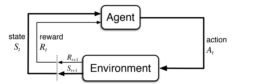
The agent (the decision maker) interacts with an environment. For example, a chess playing agent interacts with the chessboard and its adversary which is in total the environment. At each time step, the agent takes an action and applies it to the environment. In response, the environment returns a new state and a scalar reward.
It is called an episodic task (problem) if the sequence of interactions ever end with a terminal state. Otherwise, it is called an infinite-horizon or continuous task. One example for the episodic setting is chess game, in which the game eventually ends with win/lose/draw. A continuous task may be an autonomous driver agent, in which we may consider the environment as never ending.
An important concept to point out here is the Markov Property. We want our Markov Decision Processes to have such state representations, so that the state transitions are independent of the previous states. In essence, you should design your problem in a way that when the agent receives the states from the environment, it should be enough to make decisions upon them and never require a history of states. This property is called the Markov Property [2].
Models / Policies / Value Functions
The three fundamental components of reinforcement learning methods are models, policies and value functions.
Model: The mathematical representation of the environment’s changes according to agent’s actions.
For the majority of the common reinforcement learning algorithms, there is no model (model-free algorithms). This is because, the models are in some cases impossible to create or they are infeasible to use in computations.
Policy: The agent’s decision function. A policy maps states into actions, or probability distribution over actions. To better explain, you may think of the example of chess game. The policy is the function that determines what moves will be made at each state of the game.
We’ll typically denote policies with π.
Value Function: Represents the (expected) cumulative rewards starting from a state (and an action), if you follow a policy from that point on.
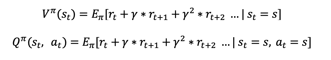
Think of the following example to better understand value functions. The environment is a chessboard game. Assume that we have not discovered any smart policies right now, so the policy is set to uniform random for any state (The actions are possible moves on the pieces). The states are the current positions of pieces in the chessboard. There is +1 reward if the agent wins the game and 0 otherwise (Realize the fact that the +1 reward only comes at the very end of the episode). The value function for any state will represent the current value of that particular state, if you follow the random policy from that point on. In the case of chess game or Go, the value function exactly represents the chances of winning the game in that state. Of course if there is a clever opponent, the agent will easily be beaten as it just uses a uniform random policy.
Also, realize that there is a parameter gamma (discount factor) in the definitions of both types of value functions. The role of gamma can be explained in two ways,
- Ensures that the value function does not go to infinity in continuous tasks
- Inserts the concept of time horizon within the scalar reward values
Gamma is always in the range of [0,1]. As gamma gets closer to 0, the immediate rewards become more important.
Control and Evaluation
After the brief introduction of the previous concepts, you may already have some idea about what reinforcement learning aims to achieve. We can discuss two tasks here to better understand the reinforcement learning process.
Evaluation is the task of estimating the value function V (state value function) or Q (action-value function) for a given policy π.
Control is the task of obtaining the policy π(a|s) which maximizes the expected sum of rewards for any state.
In state-of-the-art reinforcement learning methods, the evaluation and control tasks are very much integrated. We repeatedly interact with the environment using our policy and try to obtain a better evaluation function. With the guidance of the value functions we improve our policy in an iterative fashion.
But how do we iteratively obtain a better policy anyway, especially in such complex environments that reinforcement learning tries to tackle? Two important concepts regarding this concern is covered in the next section.
Exploration and Exploitation
As we try to improve our policy, we face an important trade-off. Should the policy dig deeper and focus on what it already learned to be good or should it explore new actions? This issue is referred to as “exploration and exploitation trade-off”.
Exploration is the process of exploring new states and new actions in order to obtain a better policy. In state-of-the-art methods, exploration is especially conducted in the early stages of the training to direct the algorithm into proper learning path.
Exploitation is the process of getting better at previously discovered and well-rewarding actions and states.
As you might guess, exploitation is more emphasized in the later stages of training.
A Brief Introduction to Reinforcement Learning Methods
As we come to the end of this article, it is a nice touch on reinforcement learning methods to better understand where the previously mentioned concepts fit in the actual algorithms.
Value Function Based Algorithms
Consider what an action-value function Q(s,a) does for any reinforcement learning environment. It estimates what is the expected sum of rewards given a state and an action. Consider a hypothetical board game where there are three possible actions in any given board position. The opponent makes a move and the RL (reinforcement learning) agent faces a state (observation). -Since we have the Q function in hand, we can see (estimatedly) what the values for each action in that state are. So, we can define our policy as: “Pick whichever action has highest Q value currently”. This policy sounds like a pretty good way to make use of our value function. In addition, it is possible to update the Q function as the agent interacts with the environment.
This idea is the basis for value-function based algorithms. A few of them are
- DQN [3]
- SARSA [4]
- Expected SARSA [4]
and many variations on top of these algorithms.
Policy Gradient Methods
What if we learn the policies directly instead of deriving them from value functions? This idea is the basis for policy gradient methods. The aim is to obtain a policy function π(a|s) directly, which maps states to actions, instead of looking at value functions first and deriving a policy from there. The fundamental algorithm for policy gradients is REINFORCE [2].
Actor-Critic Algorithms
It is a nice idea to learn the policies directly but it is better to utilize value functions that provides a guide with estimations of how policies do in terms of expected sum of rewards. Actor-critic algorithms use these both components to obtain better policies. Actor (policy) utilizes the critic (value function) to see if the taken actions yield better or worse rewards than what is expected in that state. If the rewards are better, then it is a good idea to direct the policy towards more of those actions. This idea is the basis for most of the state-of-the-art reinforcement learning algorithms. A brief list is,
- Proximal Policy Optimization Algorithms (PPO) [5]
- Asynchronous Advantage Actor-Critic (A3C) [6]
- Trust-Region Policy Optimization (TRPO) [7]
- Deep Deterministic Policy Gradient (DDPG) [8]
- Soft-Actor Critic (SAC) [9]
The list can easily be expanded as new algorithms are developed day-by-day.
Conclusion
Reinforcement learning provides an elegant and useful way to teach computers how to perform decision-making tasks. With the increases in computing power especially after 2010s, RL algorithms became feasible to be trained in large scales and in large reinforcement learning environments. With a good base of algorithms and opportunity to discover their performance on different domains, better algorithms are discovered through each day. With ever increasing interest in the area, it is clear that we’ll see even better algorithms and their utilization in broader domains.
References
[1] https://en.wikipedia.org/wiki/Temporal_difference_learning
[2] https://web.stanford.edu/class/cs234/
[3] Playing Atari with Deep Reinforcement Learning, Mnih et al, 2013.
[4] Sutton, Richard S., and Andrew G. Barto. Reinforcement learning: An introduction. MIT press, 2018.
[5] Proximal Policy Optimization Algorithms, Schulman et al, 2017.
[6] Asynchronous Methods for Deep Reinforcement Learning, Mnih et al, 2016.
[7] Trust Region Policy Optimization, Schulman et al, 2015.
[8] Continuous Control With Deep Reinforcement Learning, Lillicrap et al, 2015.
[9] Soft Actor-Critic: Off-Policy Maximum Entropy Deep Reinforcement Learning with a Stochastic Actor, Haarnoja et al, 2018.
from CRYPTTECH BLOG https://ift.tt/3yhBMFq
via IFTTT


No comments:
Post a Comment